Rockyou. Stolen passwords and how to make more of them.
Part 1, No code.
Back in 2009, a company named RockYou was hacked. This wouldn't have been too much of a problem if they hadn't stored all of their passwords unencrypted, in plain text for an attacker to see. They downloaded a list of all the passwords and made it publicly available.
This list is commonly used as a simple first step when trying to guess a password with brute force.
The world’s most common Linux distribution used for penetration testing and ethical hacking (often to make sure a company’s cyber security is up to scratch), kali Linux, comes preinstalled with the Rockyou password list. With 2,465,266 entries from one character in length to 255 characters.
Examples of entries include:
“spongebobsquarepants”, “hi”, “1234” and my favourite “stonecoldsteveaustin”.
99% of all passwords are between 3 and 14 characters in length and the first model built was focusing on the set of all passwords of length 8, allowing upper or lower case letters and numbers (no special characters).
Motivation:
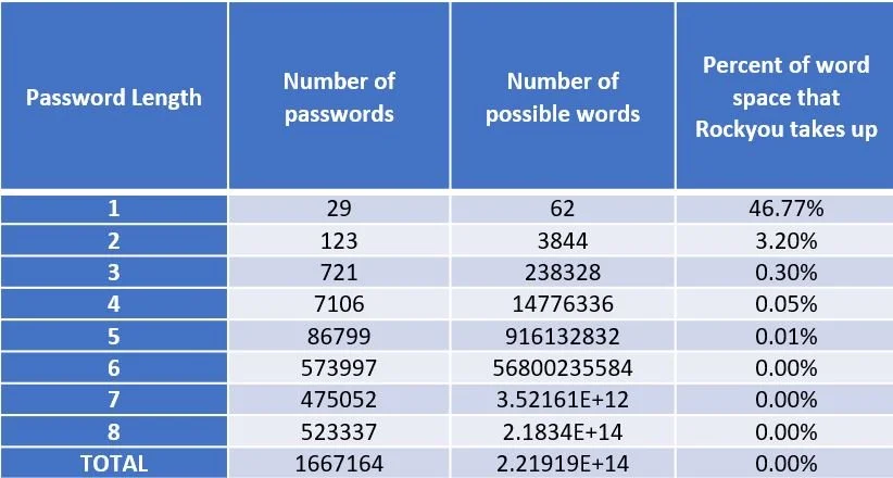
The rockyou password list is a large data set, but takes up a very small subset of all possible characters. As the size of the word increases the space that the passwords take up of all possible words of that size becomes exceedingly small extremely fast. This should make intuitive sense as most passwords for everyday logins are familiar words and patterns we can remember such as “Pink1234” as oppose to “Xt8qpV1a”. There is some structure of the data that gives it the characteristics of a password and not just a random collection of characters. If we can get a machine to learn and understand this pattern in a model that is known to be able to produce new data, we could increase the Rockyou data set with more words. This would increase the chance that you could guess someone’s password while running through the new larger data set.
Auto Encoders
Autoencoders are a non-linear dimensionality reduction model. In a simpler form, auto encoders encode or embed data from some high dimensional space into a lower dimensional space.
Like all models, an auto encoder is a function, but unlike typical regression models from the input space to a particular feature, auto encoders map from the input space to the input space.
Here the input space is a vector of 8 characters which we convert to a one hot encoded vector of length 8*62 = 496 (upper and lower case letters and numbers). Given some error function the neural network will try predict the input vector of each data point given its input vector. Upon first consideration this seems like a very easy task, perhaps consider the function:
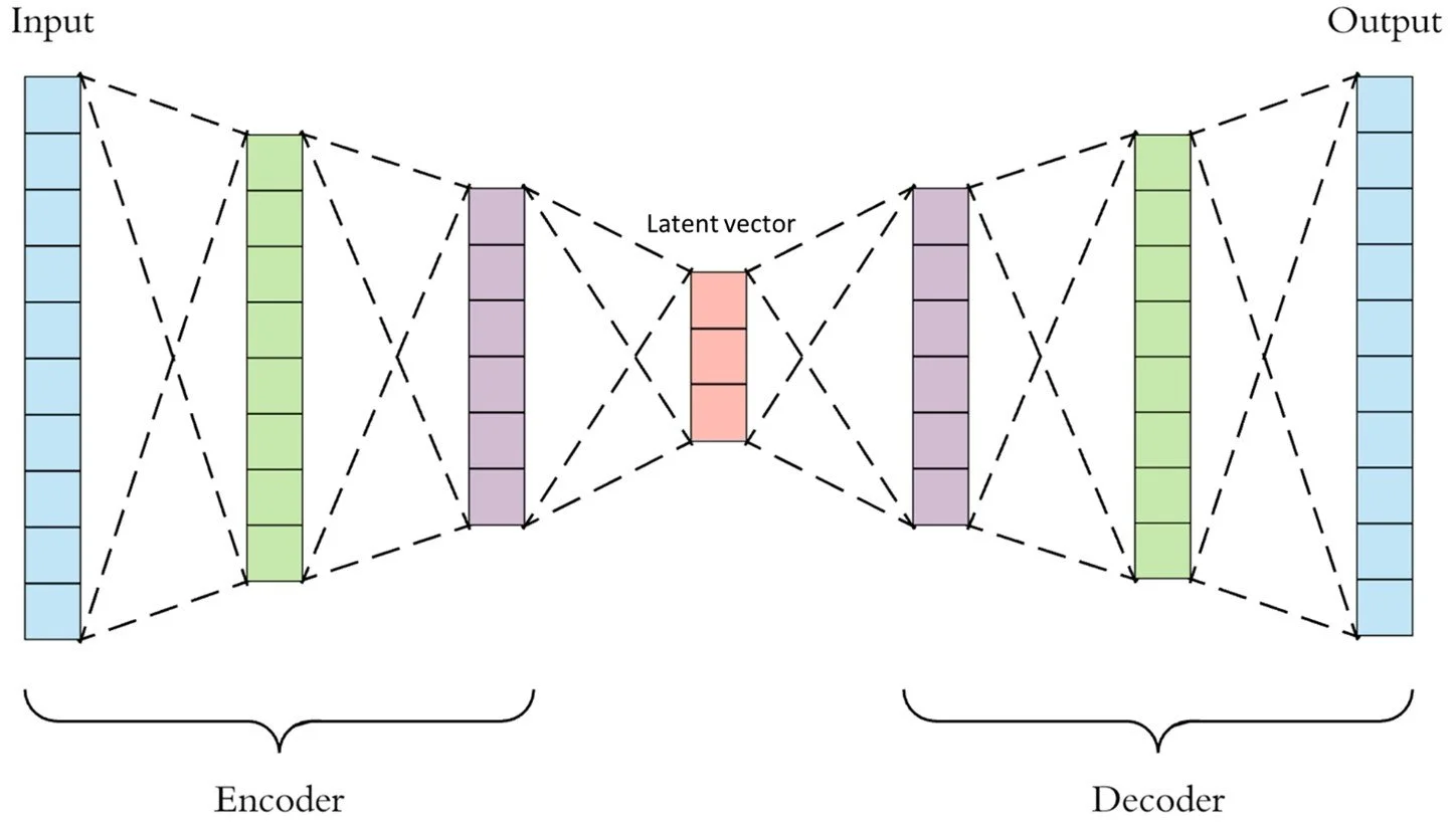
The identity function on 496 number of features. In fact any neural network with constant (or increasing) layer size can be trained on any n-data to learn the identity function. The trick of the encoder is to reduce the amount of information that can be encoded in each layer until we reach the smallest information space called the latent vector, we then reverse the process until we upscale back to the input size. By forcing the information to be lossy compressed then upscaled back to the input size the model has to learn patterns and representations of the data space in order to maximise the chance it can correctly upscale the latent space to the data space.
The smaller the latent space the more the data gets “squeezed” into a smaller vector space meaning the compression will be more lossy and higher error when upscaled back to the input space. But if the latent space is too large the auto encoder can learn the identity function without having to resort to exploiting patterns in the data. As with almost all machine learning, we want the model to learn the real-world relationships between features in the data, this makes the size of the latent space an especially important hyperparameter to tune.
How do we take an autoencoder designed for dimensionality reduction and make it a generative model?
The auto encoder can be thought as two models put together, the encoder and the decoder.
The encoder maps form the input space to the latent vector and the decoder maps from the latent space to the input space. If we sample points in a particular way from the latent space and apply the decoder to this latent vector then we will get a randomly generated data point in the input space! This means we can generate data points that have the same relationship between its features as is apparent in the original data space. This data generation technique is called a GAN, generative autoencoder network.
A quick note on hyper parameter tuning.
Hyper parameter tuning is time consuming at the best of times. Often intuition or indistry standards (aka a post on stack over flow told you so) are starting points with grid/brute force aproaches used to fine tune. Given my lack of proccessing power to use grid search with fine enough granuality to tune, I often use the following aproach.
Consider the list of hyper parameters you have, some numeric, some catagorical. Using an educated guess and some trial and error, find the ones that make the most impact, then pick the most important one and try a range of values in a loop and recored the result. Then fix this hyper parametor to the choosen minimium and move on to the next. This greedy aproach does not take interactions into account but by going though this proccess multiple times you can at least reach some sort of local minima.
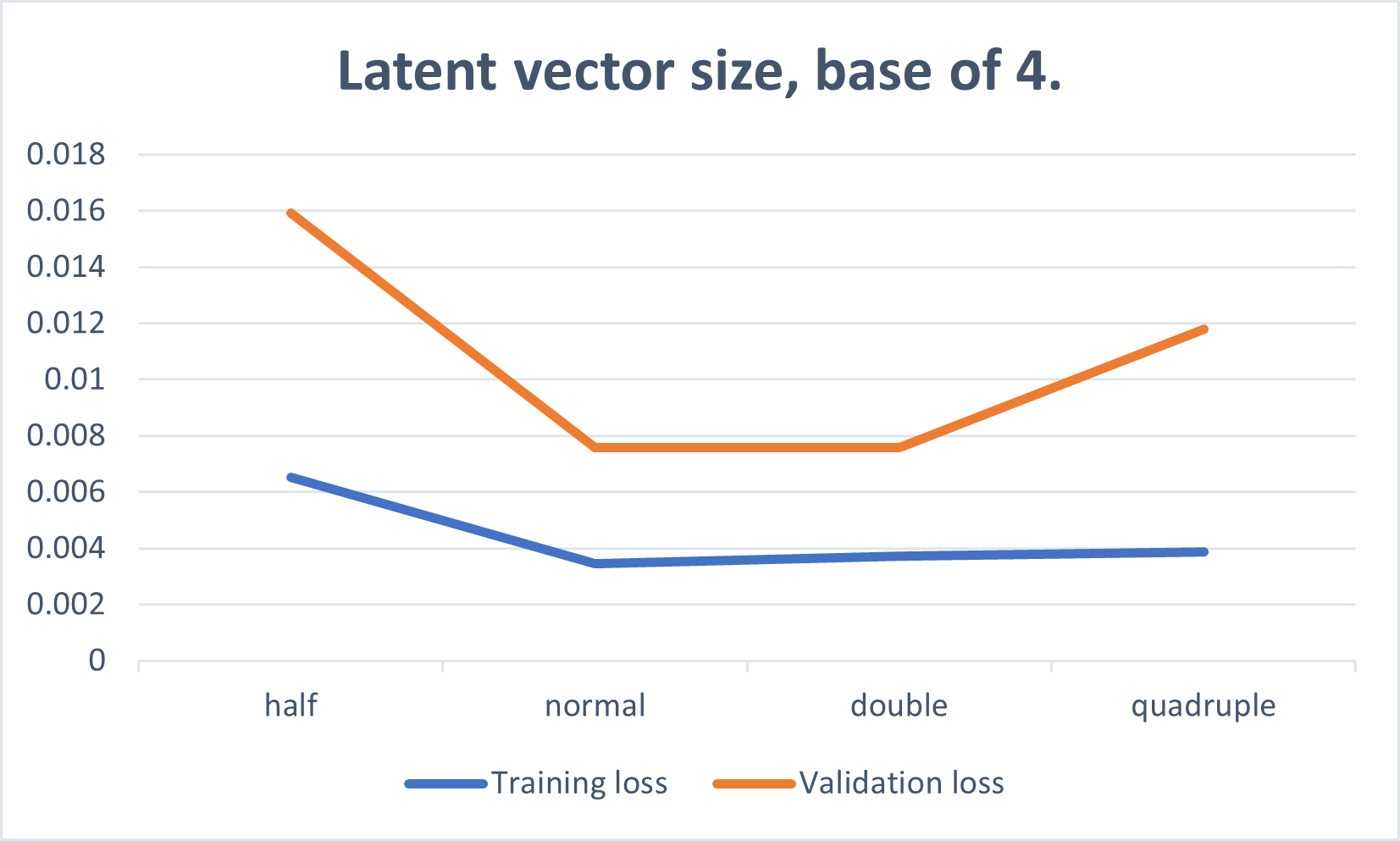
As often with neural networks, we consider everything around powers of two, this also greatly reduces the space of reasonable parameters to pick from. Above is showing how the size of the latent space effects training and validation loss.
How do we sample from the latent space?
There are at least two ways we can sample from the latent space. The first is to try force the model to populate the latent space in a defined distrabution, gaussian distribution is often the first chioce (and quite likely the last). This has it’s own set of issues, by imposing this restriction we make it harder for the model to train and find the relations between factors. We also have an issue with correlation between the vectors, we can try to also force (or measure) the copula between these, but it adds more restrictions in the model and in this case I found it untenable.
The second option is to mathematicly describe the latent space as a probability distribution function and sample from this. In practis this is done by defining buckets and to assign a probability to each bucket based on the latent space representation of the actual data then to sample from the buckets and then linearly sample from within the bucket.
Here we face the same issue that all machine learning deals with, Bias vs Variance. With more buckets we can reduce the bias but potentually overfit, while if we choose a smaller number of buckets we will underfit and more than likley sample points in the latent space that could have never come from our input data.
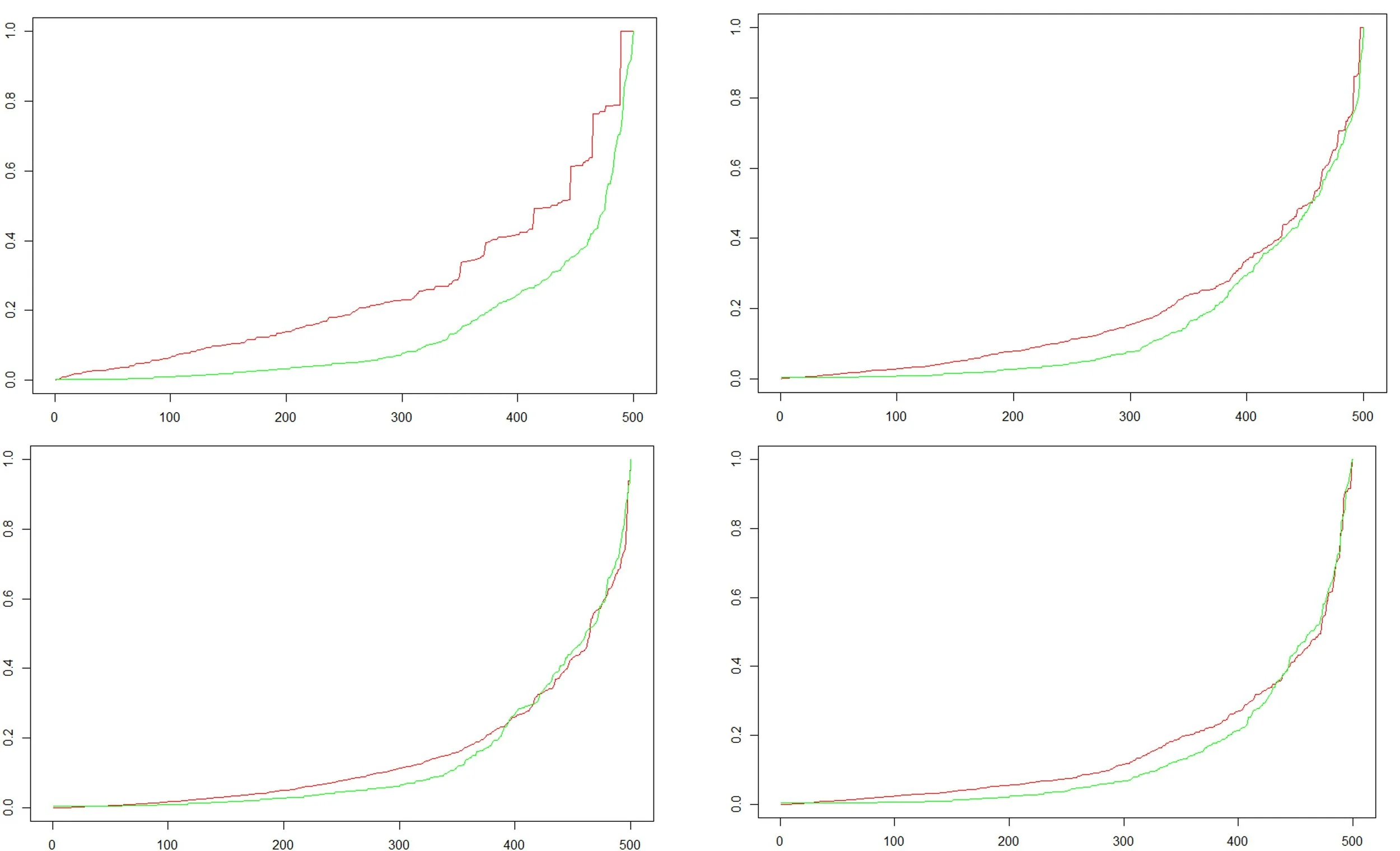
When choosing the optimal number of buckets we turn to an extreamly usefull tool for compareing two probabilty distrabutions that are complex, the Kolmogorov–Smirnov test.
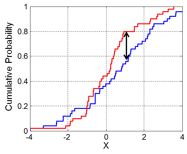
This is the final peice of the puzzle to complete this project. The idea of the Kolmogorov–Smirnov test is to generate a one dimensional distrabution of an error function, then to calculate the error on your other distrabutions (in this case, our choosen bucket distrabution) to see if it falls within your Confidence interval (or in this case, to minimise the P value).
To do this, we take a sample of our data (I choose 50%, this is somewhat arbitory but as long as it’s consistent the process is similar) and calculate the cumulative probability function. In our case with a 4 dimensional latent space we have a 4 dimensional cumulative probability function. We then take the integral between the absolute distance between the sampled cumulative probability function and the true cumulative probability function of the full data. This is our test statistic!
Example of a Kolmogorov–Smirnov test statistic.
For the number of buckets we choose the true number of buckets will be this number to the power of the dimension of the latent space. For two buckets per dimension we have 2^4 = 16 and for twenty buckets we have 160,000. Below is the cumulative probability function for buckets 4, 6, 8, 10 (in clockwise order).
I found a bucket size of 7 or 8 both minimised the test statistic and choose 7. Now we can calculate the probability of selecting each of the 2401 boxes in the 4 dimensional space by simply counting how many examples from the training data fall in each box and devide by the total.
Results!
We have trained our model on the full data after tuning it on train and test data, as well as optimise the discription of the latent space to sample from. So what happens when we sample from this latent space and decode these new data points?
herizon1, leterboo, defer1o1, sexisata, peibles1, pesswond, epilis93, riannaaa, tipper13 ,ann01010 ,heeny017 and my favourite hotgary1.
These are pretty good, it seems the model has picked up the tendency to end the password with numbers, ether a 1 or what seems to be their birth year.
Here are some lists of 4 generated passwords and 1 real one, can you guess which is which?
peter1998, peter1992, peterre93, peter1one, peterio93
91050, 85032, 20530, cora01, 80070
skak, skam, slab, slop, slot
vericon11, verizone1, verizonee, verizoato, verizon11
Answers: 2, 3, 1, 5

